CO2 gradient case study • stoic

library(stoic)

Use case

In this vignette, stoic will be used on a systems biology case study, to extract meaningful associations between:

Transcriptional profiles of genes in Arabidopsis thaliana exposed to a gradient of CO2 and two types of nitrate nutrition (KNO3: nitrate, Mix: nitrate and ammonium mix). Genes are subsetted to the genes differentially expressed by CO2 under nitrate nutrition by a spline analysis.
The TF binding scores of CO2-responsive transcription factors, scanned in the promoter regions of the CO2 responsive genes (TSS -1000, +200bp).

The fact that nitrate nutrition is tightly linked to the response to elevated CO2 has already been documented in the literature, and is very promising to uncover the pathways involved in CO2 acclimation and mineral status alteration in plants. This dataset was generated in the SIRENE team (IPSIM, 2021, unpublished).

The methodology of STOIC allows to find groups of co-expressed regulatory regions that can be well discriminated by sequence features. It does so through an exploration of the expression space where co-expression clusters are formed by maximizing the classification performance of predicting cluster membership based on sequence features.

Data import

We start by creating the data used by stoic. It needs two matrices:

The main data matrix, giving, for each observation, values in a set of samples. In our case this is, for 2092 genes, the RNA-Seq expression in 40 experimental samples (5 CO2 levels and 2 nitrate nutrition conditions). We recommend using several hundreds or even thousands of observations in stoic, and several tenths or hundreds of samples.
The guide data matrix, that gives, for each observation, a set of complementary features used to inform clustering. In our case study this is the TF binding motifs scores of 114 CO2-responsive regulators within the 2092 gene promoters. We recommend several tenths or thousands of guide features in stoic.
(Optional) The order of the samples in the main data, for visualization purposes only. In our case, this is the order of CO2*nitrate conditions to be displayed. It can be numeric or alphanumeric.

data("co2_gradient")
data <- stoic_data(main_data = co2_gradient$main_data,
                   guide_data = co2_gradient$guide_data,
                   sample_order = co2_gradient$sample_order, 
                   seed = 666)
#> The observations have been subsetted to the common
#>                     observations between guide and main data ( 2092 obs)

Running stoic

The guided clustering procedure can then be launched by stoic. Below is an example with two different initializations (nstart, as in kmeans), which are later combined to take the best clusters. We recommend increasing nstart for even more stable results (e.g 5 or more).

In this case we also lower the AUC limit to include a cluster to 0.6.

stoic_results <- stoic_clustering(data, nstart = 5, auc_thr = 0.6,
                                  seed = 666)

table(stoic_results$clusters)
#> 
#>    1    2    3    4    5    6    7 none 
#>   47   47   56   66   59   68   55 1694

The results contain several objects in a list, the most important being:

clusters: a named vector that gives cluster membership to all observations (a number, or “none” if no cluster was found in the area of this observation).
aucs : a named vector that gives the AUC (classification performance) for each cluster.
best: a list of all clusters learned by stoic, containing more details like the list of observations, AUC, the model and its predictions, the important guide features, the correlation threshold and centroid of the cluster, and so on.

Most notably, we can access the sequence feature importance of a given cluster (number 2 here) as follows:

head(get_feature_importance(stoic_results, 2))
#>     feature   importance importance_min importance_max direction
#> 1      DIV2 0.0004805618   0.0003670969   0.0005940267      TRUE
#> 2 AT5G56840 0.0004210237   0.0003038716   0.0005381758      TRUE
#> 3      MYBH 0.0003256395   0.0002311749   0.0004201040      TRUE
#> 4 AT1G19000 0.0002797340   0.0001607295   0.0003987384      TRUE
#> 5 AT2G38090 0.0002074671   0.0001115663   0.0003033680      TRUE
#> 6    NAC069 0.0001438136   0.0001045429   0.0001830843     FALSE

The direction column is TRUE when the feature has higher values in the cluster than in other observations, FALSE otherwise.

Visualization of the results

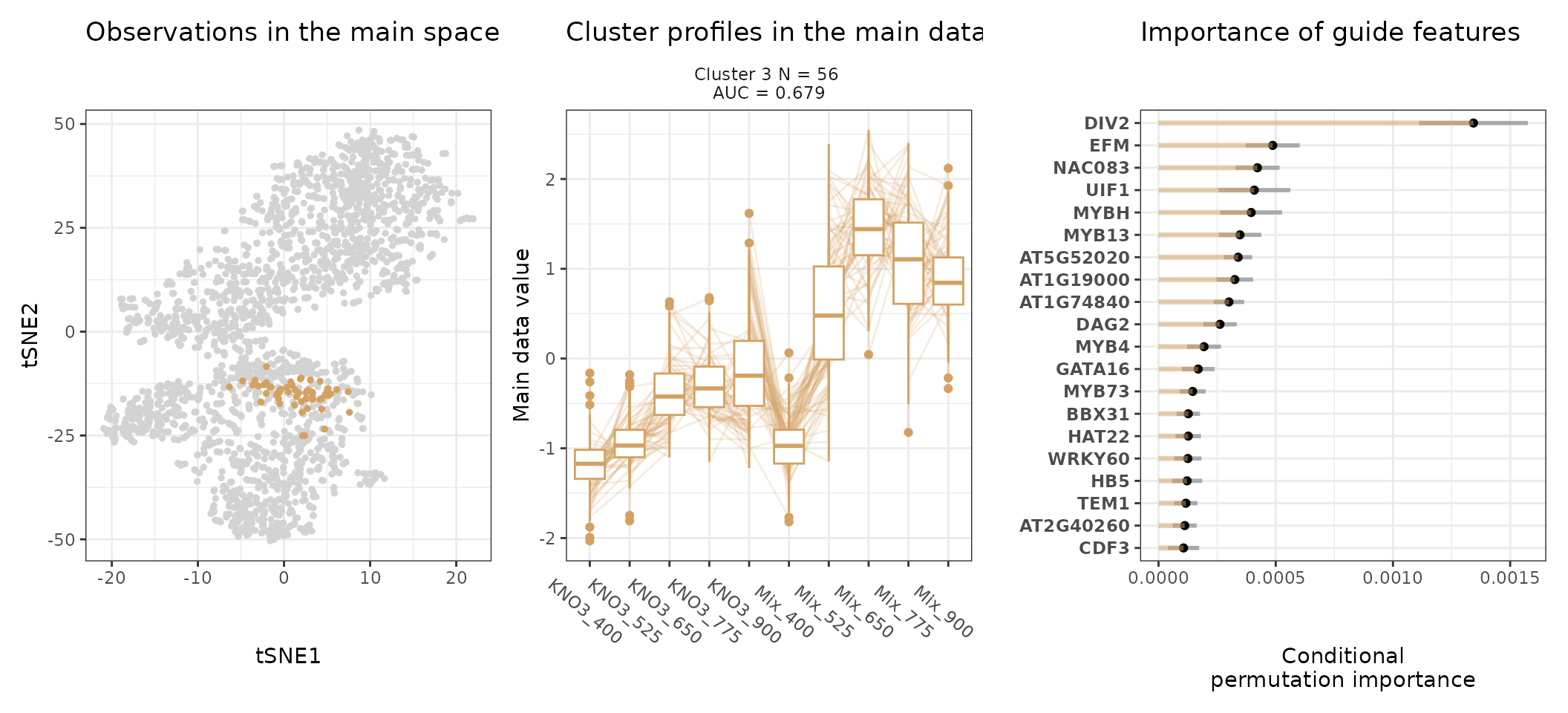
A few visualization solutions are included in the package, and are assembled together below. This gives an overview of the clustering, by showing the observations in the main space (the expression space, reduced in a tSNE), and colored by cluster. Next to it, the expression profiles of the genes appear for each cluster, ranked by AUC. Stoic here identified a series of diverse expression profiles in response to CO2 elevation (like activation, repression), that can vary depending on the type of nitrate nutrition provided. The fact that nitrate nutrition is tightly linked to the response to elevated CO2 has already been documented in the literature, and is very promising to uncover the pathways involved in CO2 acclimation and mineral nutrition alteration in plants.


draw_tsne(data, stoic_results) +
  draw_profiles(data, stoic_results)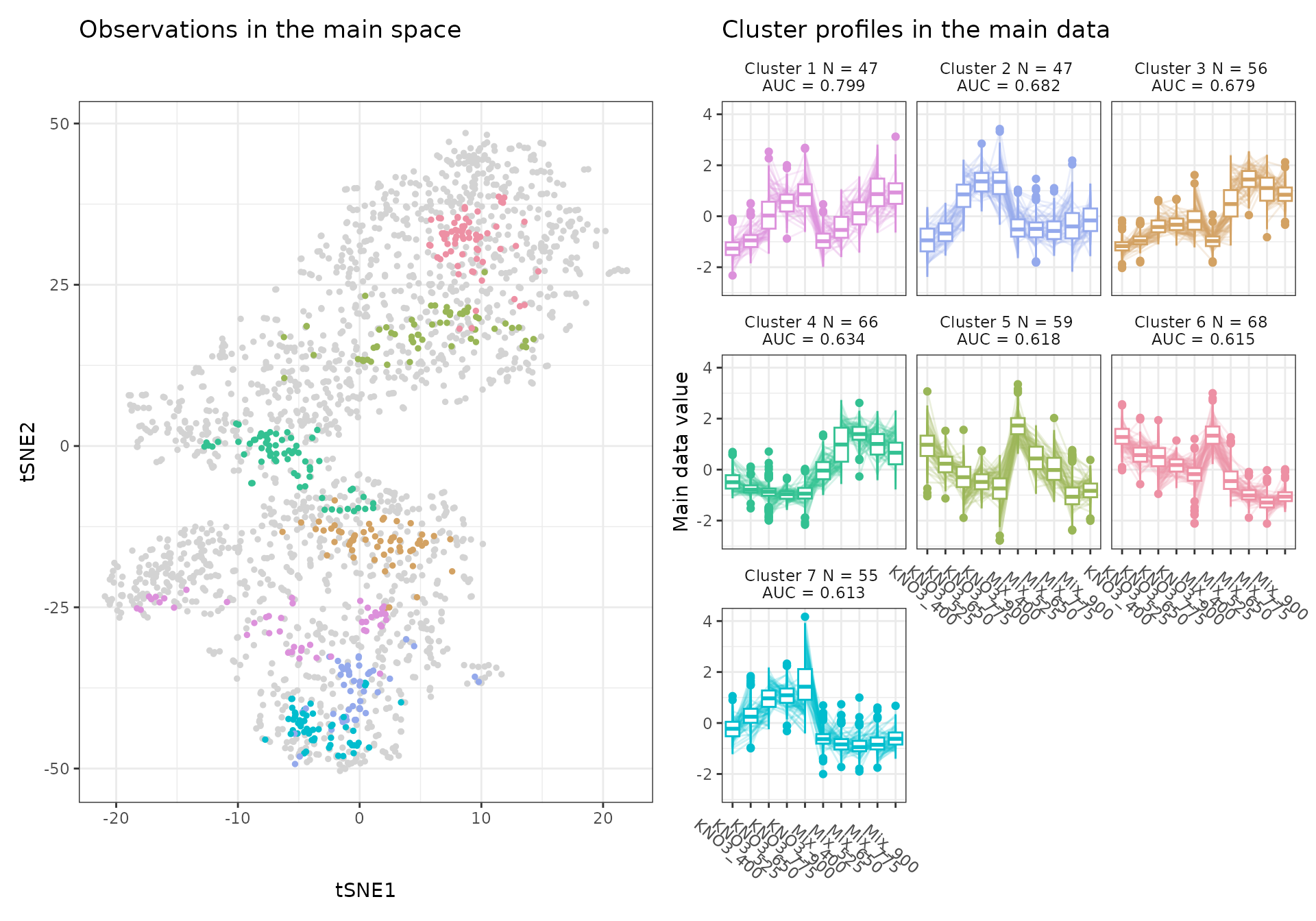

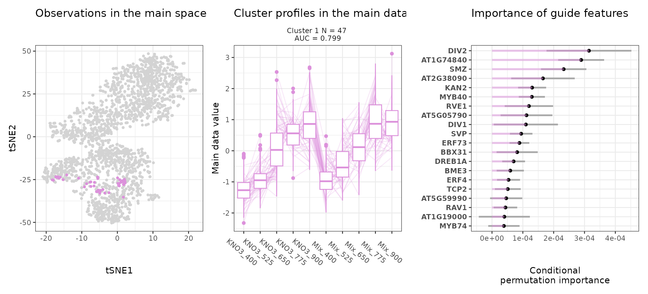
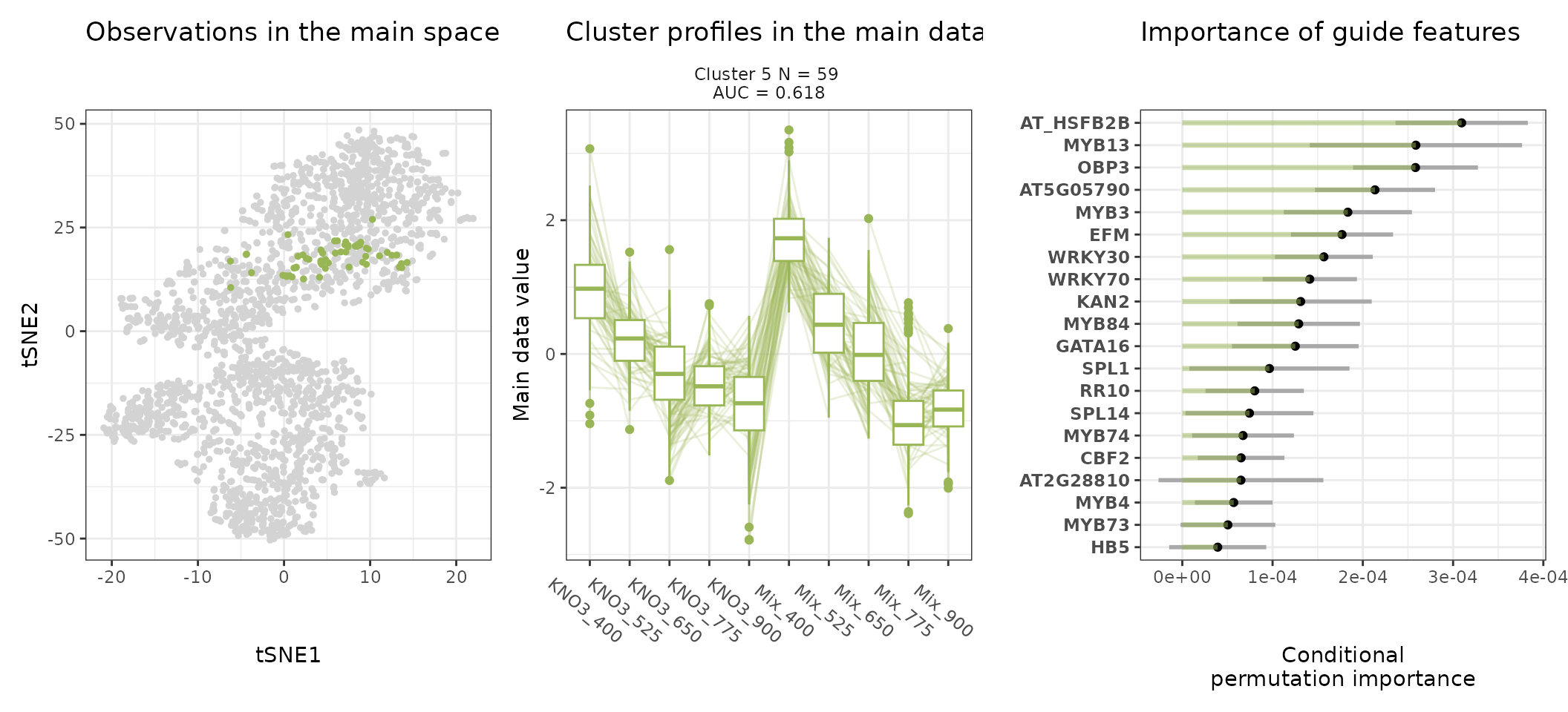
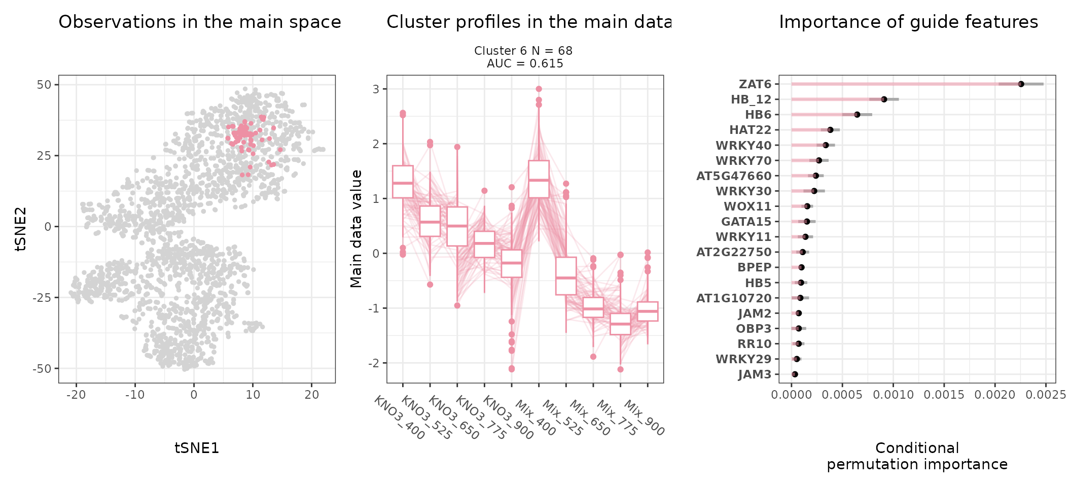
One can also look at a given cluster of interest, as in the following lines, where the important sequence features for the cluster also appear.


for (i in 1:length(stoic_results$best)){
  print(draw_tsne(data, stoic_results, cluster = i) +
  draw_profiles(data, stoic_results, cluster = i) +
  draw_features(data, stoic_results, cluster = i, only_positive = T,
                n_top_features = 20))
}

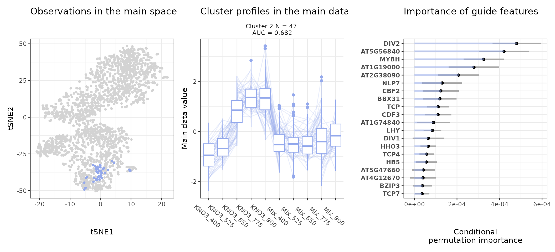
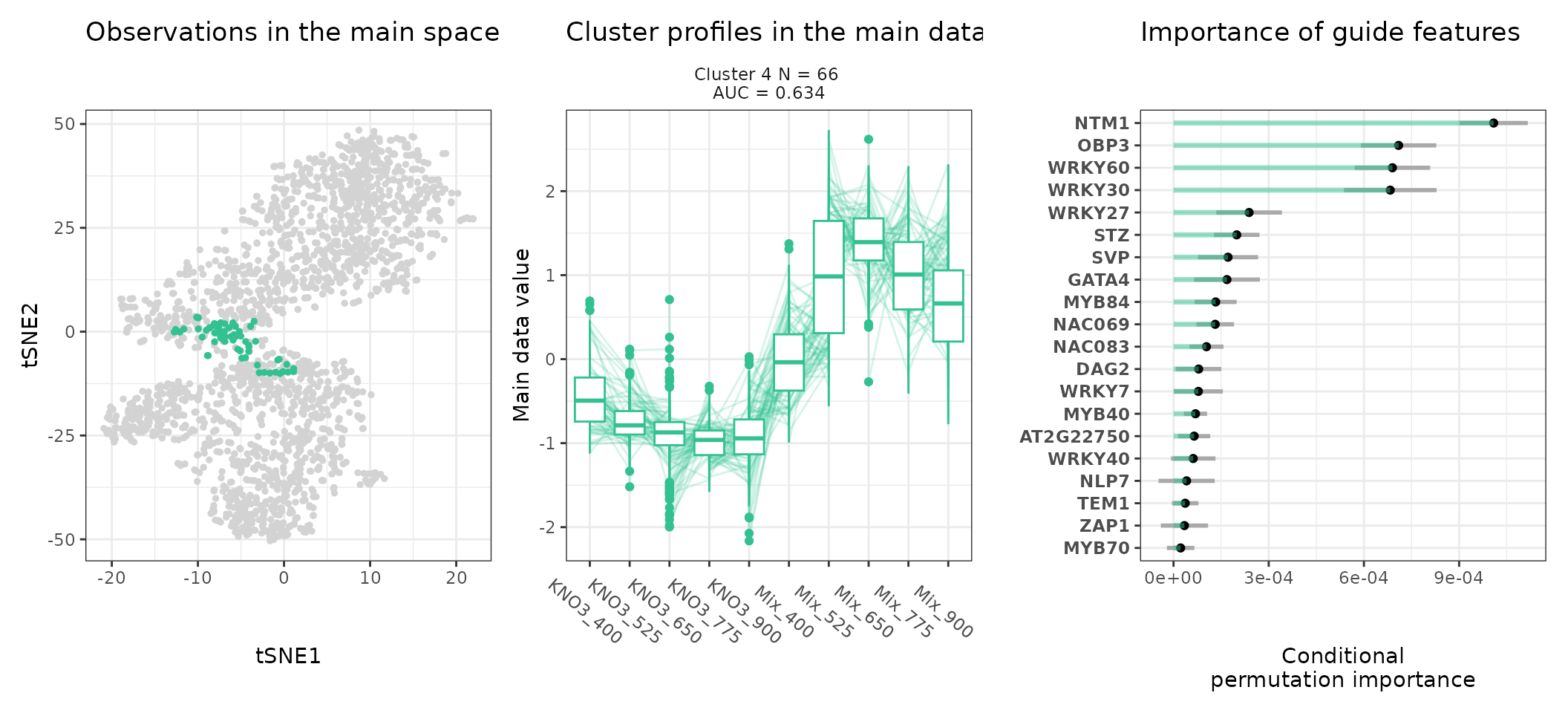
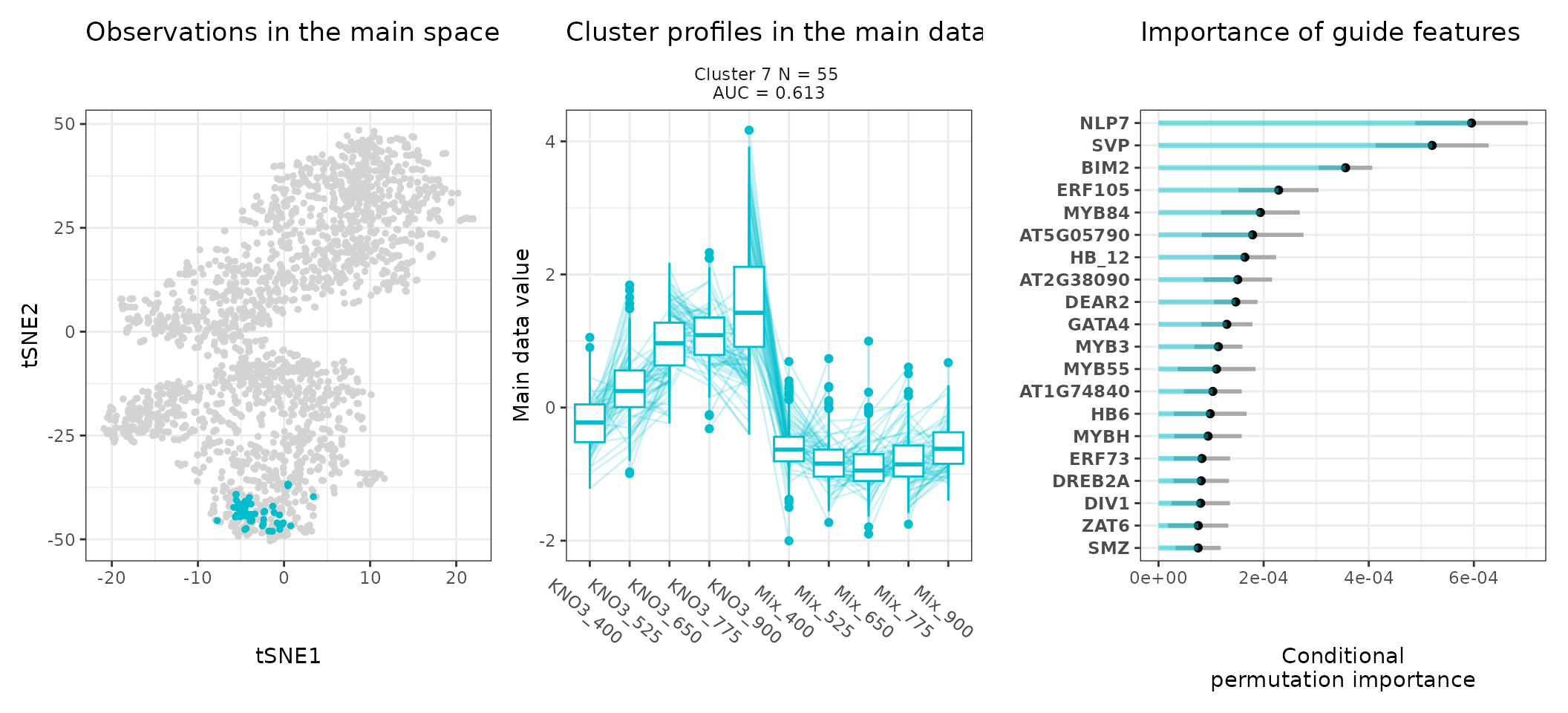
An interpretation of cluster 4 based on stoic results would be: “A set of 49 genes are mostly activated by elevated CO2 specifically under nitrate nutrition but not a mix of nitrate and ammonium. These genes can be distinguished from other CO2-responsive genes by their enrichment in the binding motifs of TFs like NLP7, DIV2, CDF3, among others. TF binding motifs, combined together, allow to discriminate these genes from others with an AUC of 0.64”.

Similarity of stoic clusters

It can also be helpful to see how similar are the inferred clusters to one another. This is done internally by stoic to prune redundant clusters, but can also be visualized downstream of the clustering. Three similarity measures are used:

A symmetrical swap score (between 0 and 1), where the model of one cluster is used to predict the membership of another cluster. It tells us weather or not the rules learned from the guide data (sequence features) are the same (score = 1), or similar (score close to 1), between two clusters.
The linear correlation of the profile in the main data (expression here), between two clusters.
The Jaccard index (overlap/union) between two clusters (the real positive classes of the clusters are considered, before the final step of assigning observations to one cluster only).

draw_clusters_similarity(data, stoic_results)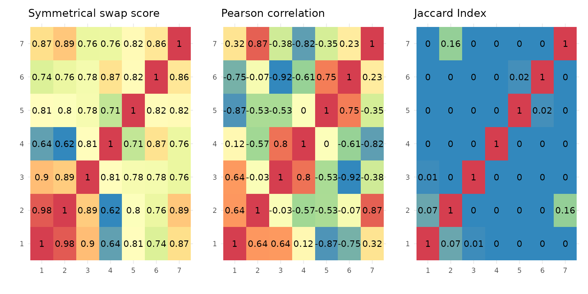

This can help the user interpret clusters, but also potentially tune the swap threshold score used in the stoic_clustering function. Clusters are deemed redundant if their swap score is above the swap threshold supplied (0.95 by default), if their Jaccard index is not 0, and if they are correlated over the maximum correlation threshold learned to define the two clusters.

Vizualize sequence features within a cluster

Stoic provides a heatmap function to show the scores of the important sequence features within a cluster (selected via an elbow rule), and compare them to observations outside a cluster. The obs parameters allow to chose whether we want to show only the observations within the cluster, outside the cluster, or all observations with an annotation about cluster information.

For example, in the 2nd cluster:

draw_features_heatmap(stoic_results, data, 2, obs = "cluster")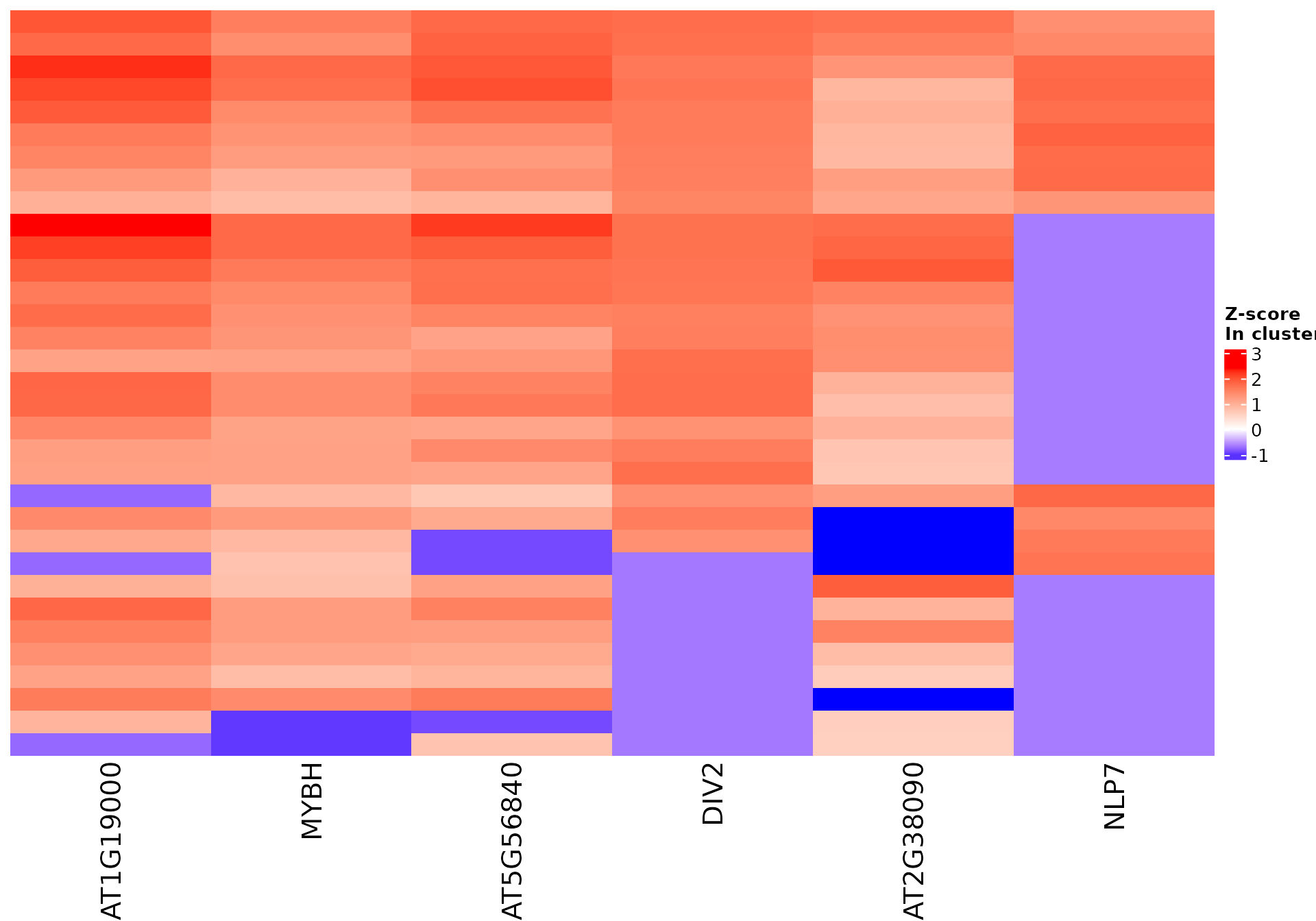

draw_features_heatmap(stoic_results, data, 2, obs = "other")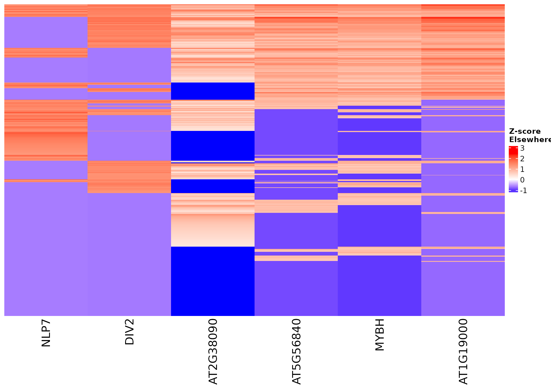

draw_features_heatmap(stoic_results, data, cluster  = 2, obs = "all")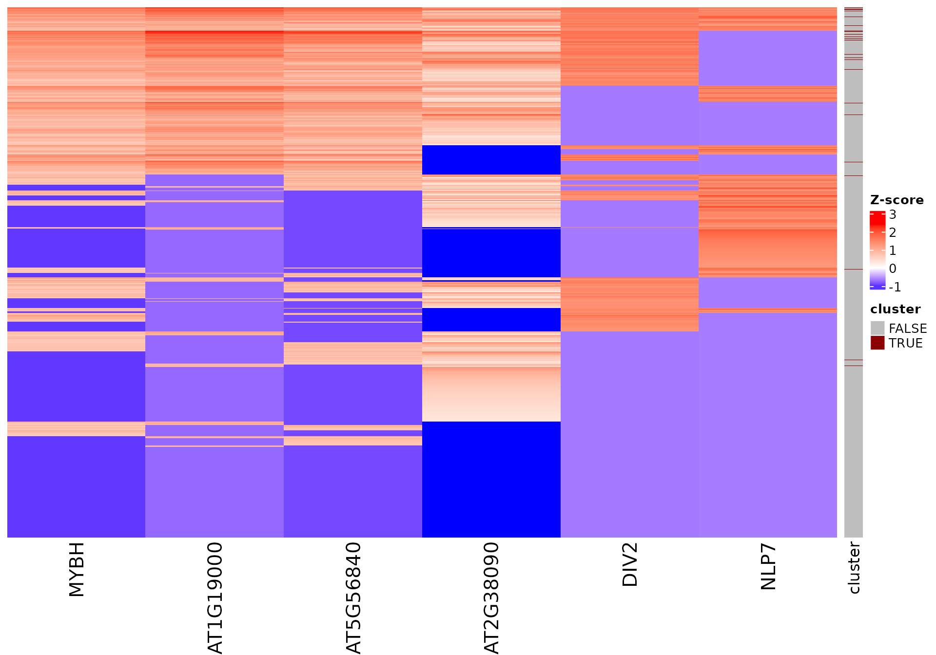

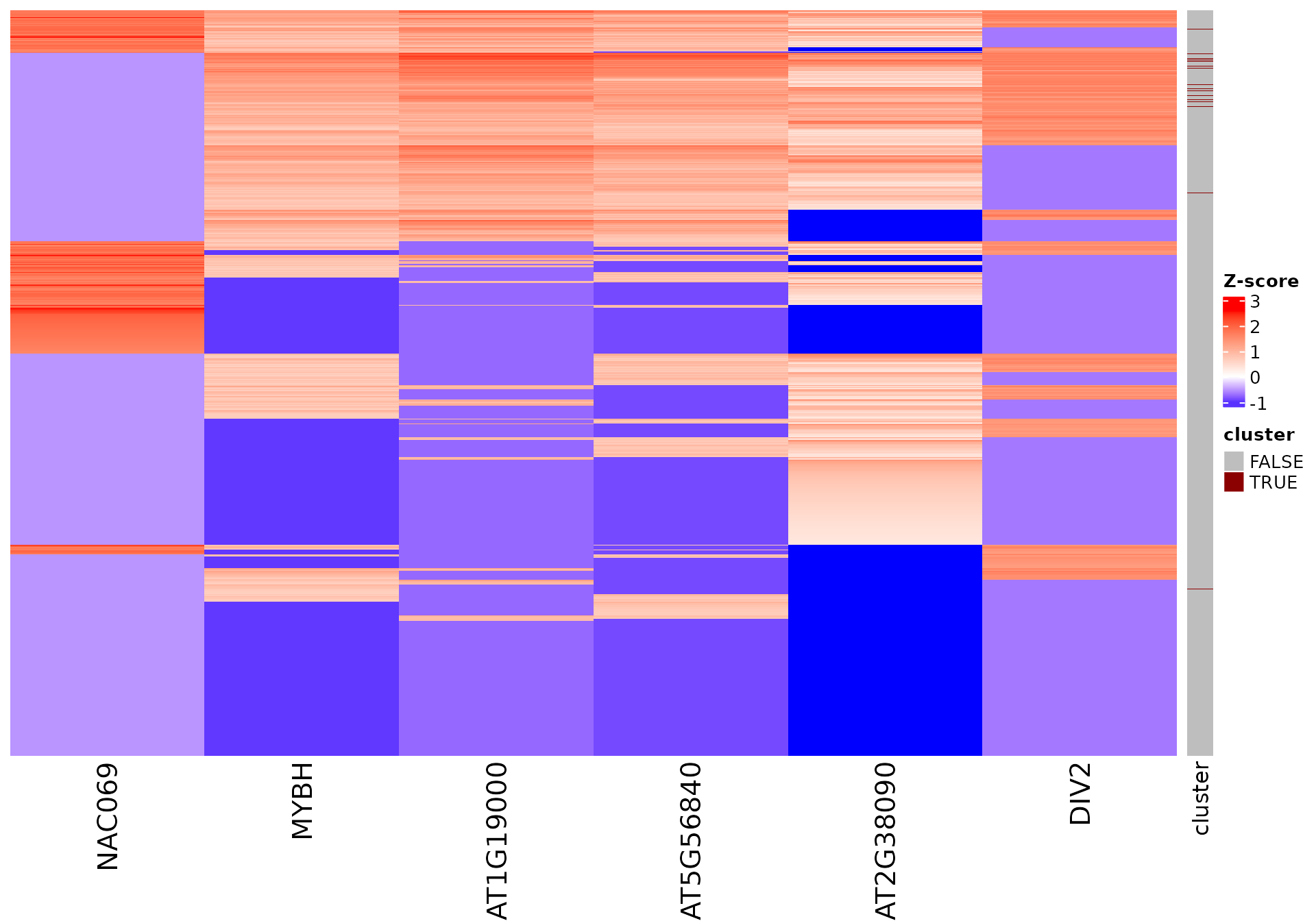
All sequence features are scaled to a z-score within all observations, so red values indicate higher than average values, and blue lower than average. By default, only the important sequence features enriched in the cluster are shown, but all important features including depleted ones can also be shown as follows:

draw_features_heatmap(stoic_results, data, 2, obs = "cluster", only_positive = F)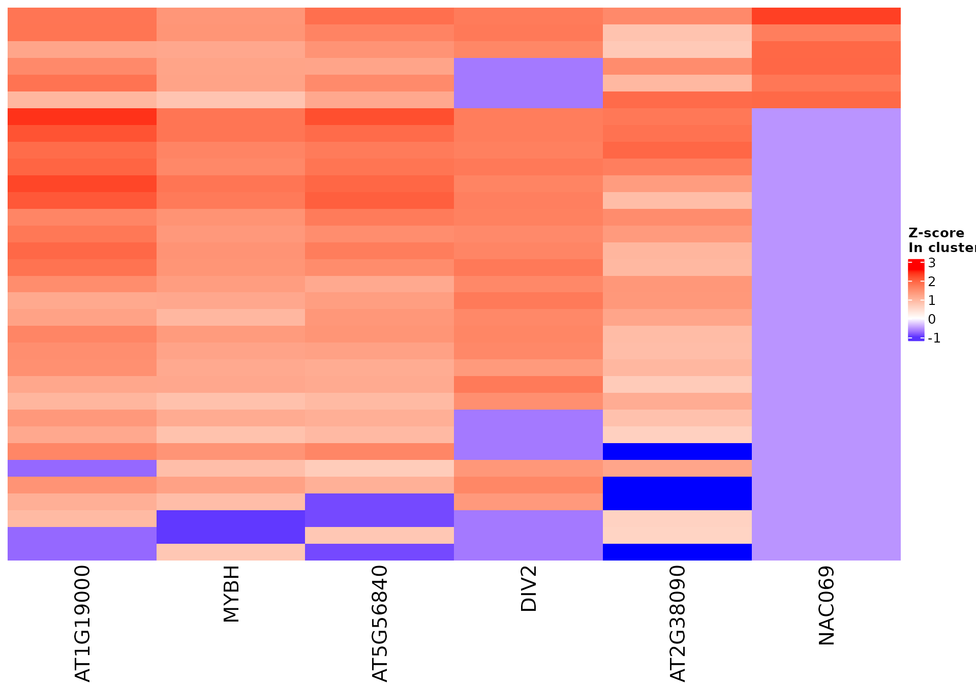

draw_features_heatmap(stoic_results, data, 2, obs = "other", only_positive = F)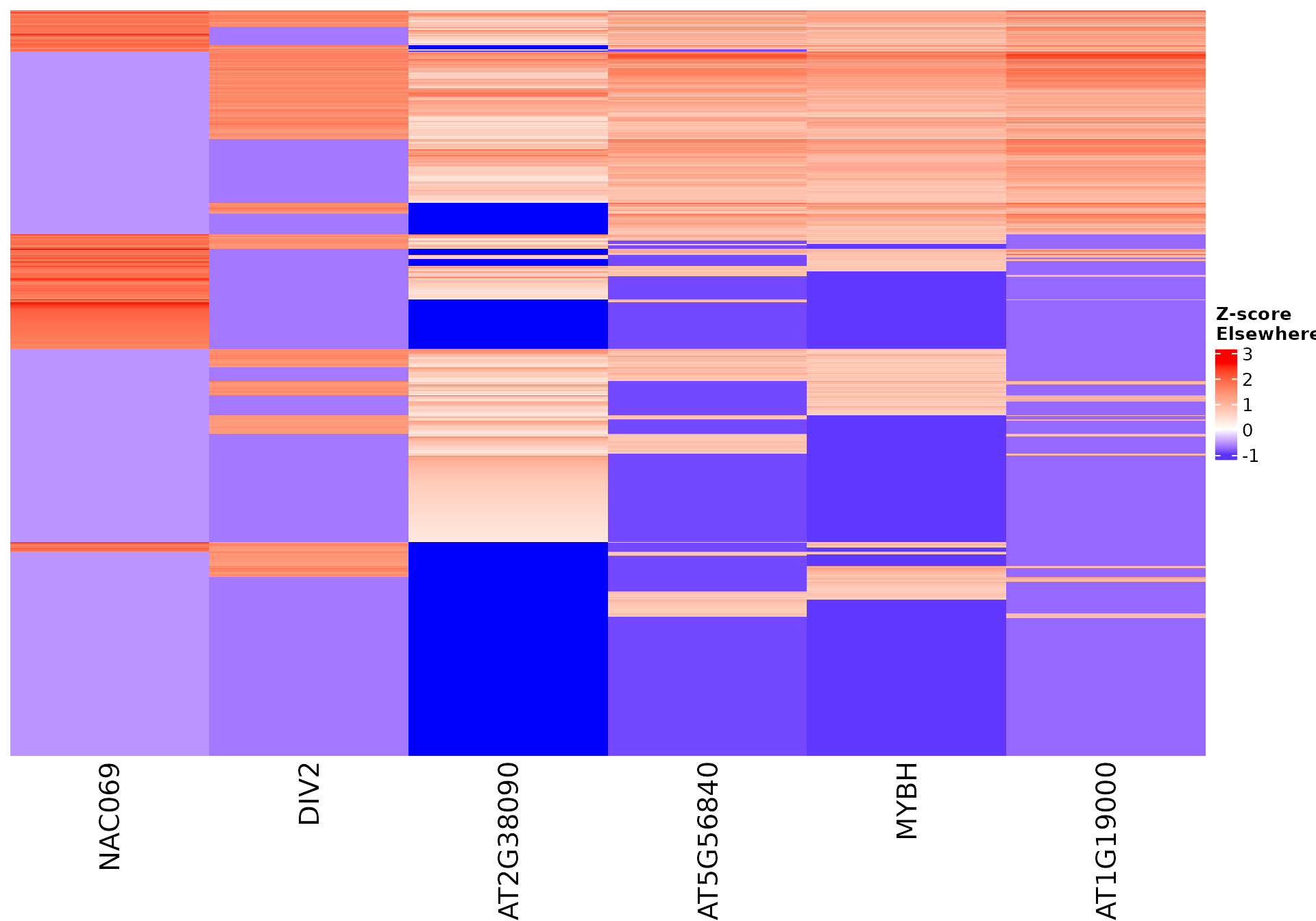

draw_features_heatmap(stoic_results, data, 2, obs = "all", only_positive = F)